C1. Fraction gaps

Sometime ago I decided that I was going to render myself a nice Buddhabrot animation to show how changing the exponent of the z-term affects the shape of the resulting point-cloud (link to video). In other words, fairly basic Multibrot stuff with z^P+c. I'd seen someone elses rendering in the past where the exponent goes from one to something like five so I had a pretty good idea of what to expect, but while playing around with the animated Multibrot it occurred to me that I had never seen an animation where the exponent goes the other way, into the negative domain. So I decided to explore that a bit, and while doing so something strange caught my eye when the exponent of z was around -1. Amid all the converging and, at least on the surface, boring point-orbits there were a handful that seemed to be diverging and producing certain distinct patterns that caught my eye. I almost thought nothing of it since at first I wasn't quite sure whether what I was seeing was just a rendering artifact caused by some bug I hadn't ran into before — the patterns certainly had that look.

Luckily however I did think something of it, but in order to concentrate on the task at hand I just made a note and threw it onto my pile of "things to look into later". And eventually I did. First by rendering a bunch of exploratory images to get a sense of what exactly I had stumbled upon. Although the image below is more stylized than the first happy accidents it manages to better capture (I think) the same structural strangeness that caught my eye on the first time around. For me the image below, when I first saw it, evoked a sense of a vast vaulted hall supported by an equally vast array of infinitely tall pillars. The vault is so high up and the floor so far below that they vanish completely and yet, a faint light shines far away in the distance. What do you see?

Forest for the Trees

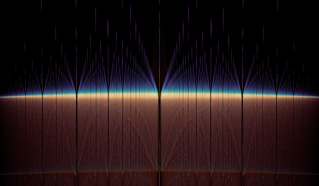
The first thing my eye was drawn to was not necessarily the patterns of light, but rather its marked absence at certain places and the blatantly fractal nature of these curious gaps — gaps where a strange synchronicity of the arrayed point-blobs conspired to occassionally line them up so perfectly that the surrounding noise simply disappears, resembling a kind of interference pattern. The widest gap in the middle of the image corresponds to c=0 with the next largest gaps to either side of it corresponding to ±i. The vanishing points at the left and right edges of the image are situated at ±2i. Practically all of the interesting orbit dynamics are located within this narrow slice of c-space. Elsewhere there are only converging orbits to be found whose dynamics are rather bland in comparison. The image is not intended as an accurate mathematical reference, but rather its main purpose is simply to visualize the gap structure we are going to be investigating. But for those interested: the vertical is a projectional blending of Re[z] and Re[c] (chosen mostly for artistic effect) while the horizontal is just pure Im[c]. Color scheme is based on the number of iterations before divergence (bluer diverges quicker).

After rendering a few more exploratory images my curiosity finally got the best of me and I started investigating whether I could find some obvious structural pattern that might explain the gaps. At this point – in the interest of simplicity – I will ditch the imaginary numbers by changing our iterated function from z⁻¹+c to -z⁻¹+c. This has the effect of shifting our interval of interest from the imaginary axis (±2i) to the real axis (±2) while preserving the proportions of the gap structure. I'm also going to omit signs for the most part since the gap structure is perfectly symmetric around zero. The reason we can get away with the former and still have the structure remain intact is due to the way the imaginary unit behaves under inversion.

We couldn't get away with this sleight of hand if we were working with the full range of complex numbers, but since our analysis is constrained to a single dimensional axis this replacement of the imaginary unit with a simple minus sign is fine. But anyway, back to the gaps.

At this point I'm still measuring things out visually which makes it pretty easy to figure out that the widest gap after c=0 and c=1 appears to coincide with √2. Which is still a nice and fairly simple number, albeit now an irrational one. A bit further out there is another gap at √3 which would start to suggest the beginning of a pattern were it not for the fact that the next square root in this apparent sequence corresponds to the vanishing points where the interesting orbit dynamics seem to cease altogether — at √4. Although in a pinch I guess you could consider the terminating points to be a special kind of "one-sided" gaps. But we'll return to them a bit later.

Continued fractions

Although we could continue our empirical measurements (as I originally did) it is more helpful at this point to start investigating the nature of the function we are iterating. It is after all the primary cause and the revealer of the gap structure. Some may consider it an obvious thing to point out, but it is something I myself realized only around this point in the story: under repeated iteration the negative exponent turns our function of choice into a fairly straightforward continued fraction. Most people have probably never even heard of (much less had the need for) continued fractions so to really drive the point home for non-mathematicians like myself, here's some visualized expansions of the function we are recursively iterating.

If you aren't previously familiar with continued fractions here are perhaps the key takeaways:

• A continued fraction is considered regular or simple if all the coefficients are positive integers (with the exception of the leading coefficient which is allowed to be negative) and the numerators of all the fractions are 1.
• A non-regular or generalized continued fraction can utilize arbitrary coefficients.
• Every finite continued fraction is a rational number and every rational number maps to exactly two regular representations (which are very similar).
• Every infinite continued fraction is an irrational number and every irrational number has exactly one regular representation.
• Finite sub-sequences of infinite continued fractions can be used as approximations of irrational numbers.

In essence continued fractions are an elegant way to represent all real numbers – the union of rational and irrational numbers – with each simple continued fraction having a certain representational uniqueness to it. As per the definitions above, our iterated function constructs generalized continued fractions since the numerators are all negative and the other coefficients (ie. values of c) are allowed to be arbitrary real numbers.

Obviously the fractional representations are more easily expressible for some numbers than they are for others, but it just so happens that the square root gaps we have encountered so far (both notorious irrational numbers since the time of Ancient Greece) have a very nice representation in the language of continued fractions. What's more, there's even an straightforward generalization that turns out to work for arbitrary square roots. However, what really blew my mind when I first saw it is how regularly the highly irregular π can be expressed as a generalized continued fraction.

De divina proportione

Something I intentionally failed to mention earlier is that when ordering gaps based on their visual width there should've been something between √2 and √3. I glossed it over because that particular gap deserves some special treatment. Included in the continued fractions above only two match the definition of a simple continued fraction. The first one is the square root of 2. The other one is denoted by the greek letter phi (Φ and φ) which is often used as the symbol for the golden ratio. Like the square roots of most numbers – and as evidenced by its infinitely fractional representation – it is also an irrational number. What makes it special is that its continued fractional form is arguably the simplest of all the infinite ones: it's ones all way down. Despite its infinite continuance it also happens to have a more compact algebraic form of (1+√5)/2. As you can probably guess, the previously undisclosed gap situated between the square roots two and three is located exactly at Φ.

The simplicity of its continued fractional form is of course not what makes the golden ratio one of the most well-known mathematical constants. As the name implies it describes a special kind of ratio which can be used to divide all kinds of things into two proportional parts. Although unequal in measure the parts resulting from this division are nonetheless proportioned in a way that some have described as 'aesthetically pleasing' or even 'divine'. In relational language this pleasant property can be expressed as follows: the smaller part is to the larger as the larger part is to the whole. A mathematically equivalent statement would be: a/b = (a+b)/a = Φ. The golden ratio has a variety of practical applications even outside the purvey of abstract mathematics.

Due to its special nature the golden ratio has a curious property which to some extent explains why it manifested itself within our gap structure: its inverse is equal to its fractional part or put simply 1/Φ = Φ-1. So simply chopping off the leading 1 from the continued fraction representation we saw earlier immediately gives us the representation for its inverse. Neat!

Thus far we have ignored the gaps that are located between zero and one, but now it just so happens that the inverse of the golden ratio matches the location of the largest gap in that interval. After this realization my overly excited extrapolation was that the simplicity of the continued fractional form somehow plays a part in how the gap structure is organized. I'm quickly disabused of this notion however as the square root gaps we identified previously aren't nearly as cooperative and their inverses (both with fairly simple representations) don't correspond to any gaps of significance. Also, none of the simple continued fractions that I try to synthesize in a brute-force fashion seem to match any gaps either.

And then?

Much to my disappointment I've pretty much run out of easily identifiable numbers at this point. The next largest gaps by my measurements are located roughly at 0.4450, 1.2470, and 1.8019, but none of these numbers mean anything to me (yet). So I make a note of the unresolved coordinates and instead start exploring the sequences of zₙ corresponding to the largest identified gaps. Considering the function we are iterating, the only way for the sequences to diverge beyond some limit is for c to be sufficiently large or alternatively for some zₙ in the produced sequences to be small. The former cannot be the case since the interesting interval is limited to just ±2 so we are left with the latter. I will let the few examples below speak for themselves.

Click to see more details

Simply by observing the value sequences we can see that each of the gaps we've identified so far seems to correspond to a repeating sequence of a certain periodicity with the lower period values corresponding to visually wider gaps. Note that for the calculations above I've chosen to make infinity unsigned to match the behavior of zero and defined the result of ±1/0 to equal ∞ and the result of 1/∞ to equal 0 (as inspired by the Riemann sphere model). You could just as well leave both operations undefined in which case the sequences couldn't be considered periodic, but they'd still possess a unique measure of length which is the important thing. This makes it possible to assign a new property to each of the gaps which will become important going forward.

Later on whenever the need arises I will refer to the gaps of linearly increasing periodicity which approach our vanishing points as the primary gap structure. This primary structure currently consists of the known numbers 0, 1, √2, Φ, and √3. So far the only one gap not belonging to this primary structure we have managed to identify is the inverse of the golden ratio.

At this point it occurs to me that the key property relating to the gap structure actually seems to be these curious proportionalities that arise from the interaction of the c constant and the inverses of the prior zₙ values. At least it is a common factor between all the gaps identified so far: the inverse of √2 is equal to half its value, Φ minus its inverse is equal to one, and the inverse of √3 is equal to a third of its value. As a degenerate case, one is its own inverse, while zero and infinity are a kind of special package deal: they play a part in all of the sequences. Their appearance is actually a necessity since earlier we concluded that zₙ has to become small for the sequences to diverge and in order for them to diverge all the way to infinity we must first pass through zero. Now, while this is all well and good it is not immediately obvious how this helps us make sense of the meaningless numbers mentioned earlier.

Got any more of them ratios?

As far as mathematical constants go the golden ratio we ran into before is probably near the top of the list in terms of recognizability with maybe only π above it. There are of course countless constants most of which are rather obscure and largely irrelevant outside a handful of very specific use-cases. However, some of these constants happen to share similar properties with the golden ratio. For example, there's a silver ratio, a supergolden ratio, and even a plastic ratio. There's also something called the metallic ratios which include the golden and silver ratios both (with 1 classified as platinum). Unfortunately none of these additional constants appear to be useful for our purposes. With the possible exception of the silver ratio, but only because it happens to include the square root of two. Instead of such a blind search we could try solving for the roots of z₅ and beyond, but the closed-form solutions tend to be absolutely horrendous. The roots most relevant to us right now are shown below (courtesy of WolframAlpha), but only as a cautionary example.

There's an upside to this madness though, as now we can pinpoint the locations of these gaps up to an arbitrary number of decimal digits! What if we just searched for the numbers on the Internet to see what comes up? It's perhaps a bit unorthodox, but our particular problem of trying to find the meaning behind seemingly arbitrary numbers seems well suited for such methods. While it is almost common knowledge that the golden ratio can be used to divide things into two aesthetically pleasing parts, up until this point I had never considered that there might be an analogous way of dividing things into three pleasantly proportioned parts! And yet that's exactly what my search found, the not-so-well-known relative of the golden ratio: the golden trisection.

Unlike the golden ratio which is just a single constant its trisectional counterpart is defined by a pair of proportionality constants: ρ≈1.8019377 and σ≈2.2469796. The first constant clearly matches the location of our current gap of interest, but the second one appears to be beyond the interval of inspection. However, it doesn't take too much effort to figure out that its fractional part looks familiar and that all we need to do is to subtract one from it to arrive at a gap value matching one of those horrible roots above. With some further trial and error we find that the inverse of the larger constant matches the third and last z₅ root we are after. Curiously enough both of these gaps can also be represented in an alternate way: σ-1 = σ/ρ and 1/σ = σ-ρ. Recall the similar relation of the golden ratio: 1/Φ = Φ-1. It seems like we are definitely onto something!

Of course, the golden bisection and trisection are just the beginning. Rather conveniently it turns out that the proportionality constants of these so-called optimal N-sections match the diagonal lengths of certain regular polygons with side lengths equal to one. The optimal bisection corresponds to a pentagon, the trisection corresponds to a seven-sided heptagon, the quadrisection corresponds to nine-sided enneagon, and so on and so forth.

Constructing proportions

Knowing the connection between the proportionality constants and their specific polygons makes defining precise values for the constants a matter of pure geometry. In the image below each polygon encloses within itself a number of triangles with two sides of equal length, with that length matching the value of a particular proportionality constant. All green triangles correspond to a proportionality constant of 1 which could be considered to be the first constant of each optimal section. Something to which everything else is in proportion to. However, for convenience I will reserve the label first for the first constant larger than one (at least in this post).

The top angles for all these proportional triangles found within a single polygon are the same with the angle magnitude shown as a fraction of π. Likewise, the magnitude of the internal angle of each polygon is also shown on their left side. Due to symmetry there is nothing special about the chosen orientation of the contained triangles. They could just as easily be constructed starting from any of the other vertices. Indeed, the dotted lines in the diagram that trace out the bases of the colored triangles also show the outlines of an alternate set of equivalent triangles which are rooted in bottom left vertex.

Figure 1: Odd polygons

Knowing the equivalences and just these few angles it is possible to figure out all the rest. Then, by applying the sine theorem the lengths of sides opposing the known angles can be derived. Showing all the intermediate steps is beyond the scope of this post, but the derived values for each constant are shown below its associated polygon. For the first constants the ratio of sines can be simplified to a single cosine which can be generalized to 2cos(π/k) where k indicates the number of corners in the polygon. The relation between the optimal N-section and its polygon is given by k=2N+1 with the equilateral triangle (k=3) providing the degenerate case of N=1 — the optimal way to divide something into one is to not divide it at all.

Admittedly, this fairly straightforward geometric construction of the proportionality constants is something I figured out only as I was drawing these diagrams (better late than never right?). Although the page on the golden trisection I found earlier did contain a similar construction specific to the heptagon, at that time I figured that working out the constants for other polygons by purely geometric means would be way too tedious with my rusty skills and that an easy generalization probably would not be forthcoming. Which is why I initially derived the values of the proportionality constants via rather different and in hindsight, more cumbersome, means. Why this initial geometric laziness paid off in the most surprising ways will become apparent in the next post.

By plugging some of these newfound constants into our continued fraction formula it quickly becomes apparent that the number of corners in the associated polygon matches the periodicity of the generated fraction sequence! Perhaps even more surprisingly the generated sequences can be defined entirely in terms of the associated proportionality constants. Rigorous mathematical proof for these statements is left as an exercise for the reader though. Some of the leaps made in the formulas below can also seem somewhat non-obvious (at least for now), but they can be easily verified numerically — the analytical verification doesn't quite fit into the margins.

Click to see more details

At this point another curious pattern begins to emerge which is worth pointing out, this time in the value sequences of zₙ. Looking at the results above (as well as the ones from earlier) we can see that the number 1 only makes an appearance in sequences that have an odd periodicity. In other words, it only appears in sequences associated with an optimal N-section while being markedly absent from the even-period sequences resulting from c=0, c=√2 and c=√3. In addition, a neat sequential symmetry arises around it: notice how the values that come before it are repeated in reverse order and in inverted form after it. This same symmetry also applies to the even periodicities although for those sequences the symmetry mid-point is located "between" the iterations, eg. √3/2 is immediately followed by 2/√3.

Evening things out

As alluded to earlier the optimal N-sections only provide us with the gap locations of every other periodicity (due to k=2N+1) which has left the gaps corresponding to even periodicities unaccounted for. But in fact we have already inadvertently solved the general problem, at least as far as the primary gap structure is concerned. You can probably guess why if you consider the shortest diagonal lengths of the unit square (√2) and the regular hexagon (√3). Indeed, the gaps of even periodicity are associated with their own set of polygons for which the polygon-periodicity relation is equally true.

Conveniently the way in which we calculated the lengths of the shortest diagonals (ie. first proportionality constants) applies generally for all polygons. Which means we are free to use the same 2cos(π/k) formula to derive the primary gap location for any periodicity k. Even more generally the lengths of all the diagonals of all regular polygons with a side length of one can be produced by sine ratios similar to the ones we saw earlier, the 2cos(π/k) being just a simplification of the first case. However, unlike the diagonals of odd-cornered polygons the longer diagonals of the hexagon, octagon, and other even-cornered polygons seem to play no significant role in the gap structure even though they do possess their own kind of beauty (note the appearance of the silver ratio!).

For the time being let us concentrate on the primary gap structure, or in other words, on just the shortest diagonals. As we calculate some of them out yet another pattern seems to arise. However, this time the pattern is not linear in the sense that the previous ones have been, but instead what we find is a periodic doubling pattern. At the limit, when k goes to infinity we reach our vanishing point at 2. The implied doubling pattern allows us to derive a neat infinitely nested radical representation for it.

First verifying some of these visually and then by plugging them into the continued fraction formulas they all seem to check out. Although again, rigorous mathematical proofs are beyond the scope of the post. At this point we have pretty much figured out the positional pattern of the entire primary gap structure. It can be neatly compressed into a simple trigonometric formula parametrized only by the periodicity of the associated continued fraction. This formulation turns out to have some interesting implications. From the equations above we can see that the vanishing points at ±2 correspond to fraction sequences of infinite periodicity. As the period becomes infinite the sequences become (at least in practical terms) aperiodic and converging. Since we are only analyzing the diverging sequences this transition point between divergence and convergence naturally coincides with the end of our gap structure.

Note that convergence and aperiodicity do not necessarily go hand in hand as it is perfectly possible to have non-periodic, and non-converging dynamics. But for us this is not the case and beyond our initial interval of inspection in the domain of convergence the infinite continued fractions acquire singular well-defined values. At the vanishing point as n goes to infinity the value of zₙ approaches 1. In our finite real-world domain however, the approximation simply improves with increasing n never quite reaching exactly one. Far from being boringly uniform as I originally thought there are some cool dynamics to be found even amidst these converging sequences. Where have I seen those faint branch structures before ..

So, in addition to the linear trigonometric pattern of the primary gap structure we have also found a doubling pattern which is period-agnostic and cares only about the gap position — simply by knowing the location of a gap we can find another a bit further out. The only thing it tells us about the underlying sequences is that their periods will have a two-to-one relation provided they are both part of the primary structure. Somewhat later I managed to figure out that there are also analogous patterns of tripling, quadrupling, etc. which generalize (very impractically) ad infinitum, but that's something I need to save for a later post. Lastly, since the trigonometric formula is invertible we can derive a function which given a primary gap location can tell us the periodicity of its continued fraction sequence. So in summary, our knowledge of the primary gap structure can be stated in the following way.

The fact that the dynamics of our continued fraction formula manage to squeeze an infinite parameter-space within a finite interval implies that the structure is in a certain sense hyperbolic. Simply put, there's somehow way more stuff located within this small area than our linear common-sense makes room for. Something which is also beautifully captured in the works of M.C. Escher. Hyperbolic spaces and fractals tend to go hand in hand because fractals are in visual terms displays of infinite structure compactified within a finite linear space (fit for human eyes). This is merely an artifact of representation though since it is certainly possible to have something infinitely complicated also within an infinite space — a universe onto itself. Although real-world physics tends to impose certain resolution restrictions. In any case, this leaves us with the problem of the secondary gap structure, or structures, depending a bit on how you look at it. Luckily we already have some clues.

Gaps between gaps between gaps

The gaps we currently know of that do not fit within the primary structure are located at σ-ρ, σ-1, and Φ-1. With some trial and effort we can manufacture more similar combinations from the proportionality constants we calculated earlier. From the period-9 constants we can derive gap locations for γ-β and β-1, while the period-11 constants give us coordinates for μ-λ, μ-κ, λ-θ, and κ-1. The even-sided polygonal constants follow their own peculiar logic although the values aren't quite as neat since everything seems to be wrapped within square roots. At this point we should probably visualize what we have found so far. In the annotated image below for each gap highlighted in red its periodicity is shown above and its exact location is shown underneath. The primary gap structure gets a bit crowded at the hyperbolic right edge.

Figure 2: Forest of Annotations

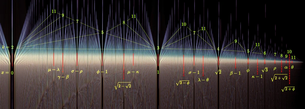
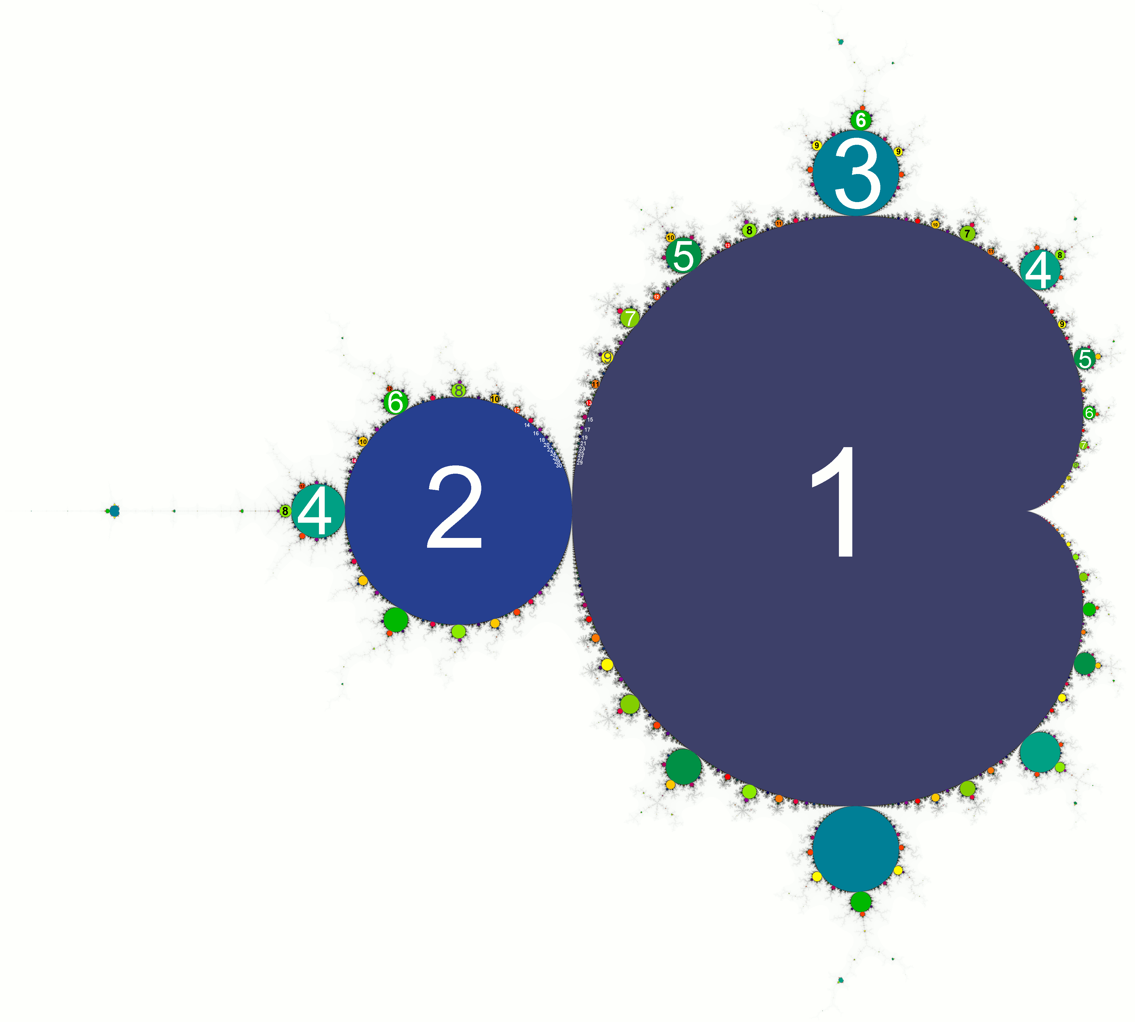
There is a very definite order to the way the gap periodicities are distributed. In a remarkably straightforward way the secondary gaps are kind of built on top the primary gap structure and the periodicities turn out to be sums of the adjacent periodicities: 5=2+3, 7=2+5=3+4, 8=3+5, and so on and so forth. This requires us to define adjacency in a non-positional way though: A is considered left-adjacent to B if it is the first gap to the left of B that has a lower periodicity than B. Substitute the "lefts" for "rights" and you get the equivalent statement for right-adjacency. If you squint just right this triangular summing pattern seems to resemble the branching structures we found in the convergent dynamics. The relation to the bulb-periods found along the perimeter of the main cardioid of the Mandelbrot set also becomes rather clear. Unfortunately this pattern only applies to the periodicities of the continued fraction sequences. No such simple pattern is forthcoming for the locations of the gaps which – as we saw earlier – are the rather complicated roots of particular polynomials.

This sum-pattern conveniently happens to offer an explanation for why there are no secondary gaps associated with √2 or √3 — the monotonically increasing primary gap structure and the emergent inbetweeners seem to offer no gap adjacencies for which the periodicity sum could be 4 or 6. We could even try to shoehorn the primary gap structure into this recurrence relation provided we reinterpret the periodicity of the vanishing points to be 1 instead of infinite (so that 2=1+1, 3=2+1, 4=3+1, and so on). Although at first this sounds like an unreasonable leap, the Mandelbrot set image linked to above would certainly seem to hint at such an equivalence. Is there a way we could justify it mathematically?

Rational periodicities

Recall the k(x) function we derived earlier. Although at first glance it should seem to be valid only for the gaps belonging to the primary structure it turns out to work for all gaps, just not quite the way we intended. At first when we try to apply the function to the secondary gap structure the results appear simply incorrect (what does a non-integer period even mean?), but rather quickly a pattern seems to suggest itself. To make it obvious all we need to do is convert the decimal representations to equivalent rational numbers. Much nicer don't you think?

Notice that some fractions seem to be missing from the patterns above. The omissions are more pronounced for the even numerators whereas only 9/3 seems to be missing for the odd ones. Additionally the patterns seem to cut short since the values are always greater than 2. In our initial interpretation this was to be expected since there seemed to be no way for the periodicity of any continued fraction sequence to be less than that with c=0 corresponding to the minimum.

To complete the patterns we must reconsider our previous derivations. Unlike the cosine function which is symmetrical around zero its arccosine inverse (cos⁻¹) is not. In our formulation of k(x) we restored this symmetry rather forcefully by taking the absolute value of x thereby discarding its sign. Had we not done this we would have gotten unjustifiable results for negative values of x. However, now that we have the proper context to make sense of these unexpected results let us keep the sign and see what we get.

This still leaves us with some missing rationals. Luckily we have enough examples to see that all of them simplify into fractions which we have found. So if we really strive for completeness we can recover and place all the missing fractions as shown below. This also offers up a nice explanation for their absence: the missing fractions were simply hidden within other more prominent gaps! Perhaps this overlap (or constructive interference) is precisely what gives the gaps their prominence in the first place. The c=0 gap is the largest simply because half of all integers are divisible by two while only a third are divisible by three, making c=1 slightly smaller in comparison. This line of reasoning gives us the mathematical justification for the curious dual nature of the vanishing points.

This newfound knowledge allows us to define our gap structure functions in a more comprehensive way. By preserving the sign-symmetry of x, all gaps (with the exception of c=0) become associated with two periodicities of which one is a natural number and the other is a rational number. The periodical doubling pattern we figured out earlier turns out to apply wonderfully well also to these rational periodicities. What's more, simply by inverting it we can derive a halving function which previously would have been of only limited use, but with our rational generalization it is now considerably more useful.

Note that in the case of k(x) below the resulting value is not necessarily rational since if x is non-algebraic then its associated periodicity should be irrational. Although that's just my initial intuition which should be taken with a grain of salt. If we were to venture beyond our interval of inspection we would also need to consider what an imaginary periodicity means. Which is something best left for another time. So to re-summarize the rules of the algebraic gap structure — primary as well as secondary.

By introducing suitable sign symmetries also for the doubling and halving functions we get well-defined behaviour that matches our other formulations. If we want just a singular answer we first need to decide which of the two periodicities associated with the gap we wish to double or halve. One thing the halving function also makes possible is the extrapolation of periodicities less than one. It also happens to offer an additional confirmation of the dualistic nature of our vanishing points since H(0) = H(±2) = ±2. Since periodicities less than one coincide with the existing structures they don't offer us much new insight, so in the interest of brevity I'll skip over any examples.

Instead I want to show a different kind of (partial) representation¹ that combines some of the various ways we have so far used to make sense of the gap structure. On the top of the diagram below you can see the geometric sum-triangle formulation with the periodicity numerators labeled alongside the gap points. Note that the vertical axis is completely synthetic and the two-dimensional structuring doesn't actually signify anything concrete (at least intentionally). It is simply a neat way of uniformly visualizing the underlying branching structure which would otherwise be squashed onto and hidden within the horizontal axis. Below the horizontal axis the gap locations corresponding to the various fractional periodicities are shown which reveal the same branching pattern, but from a different perspective. In the interest of readability only the "right-handed" cosine values are shown — those corresponding to +2cos(πn/k).

Figure 3: Branch triangles

Polynomial bonus

There's just one last detour that I wish to make before wrapping things up. Although I didn't go through it in much detail previously it can be shown that every finite continued fraction zₙ we calculate can be simplified to a ratio of just two polynomials. Our detour concerns these polynomials, ones we so hastily decided to abandon as soon as we saw the horrible closed-form solutions of their roots. Since those roots are necessarily the same as the values produced by our cosine formulation we know that horrors of the closed-form representations are due to the underlying trigonometric functions. Only in certain special cases do the values evaluate to something algebraicially easy. Almost all of these structurally simple representations are radicals nested around some initial value of x — as evidenced by our period-doubling function. The simplest roots of all are associated with power-of-two periodicities that are produced when the doubling-function is recursively applied to c=0. Starting the doubling from c=1 comes as a close second. Unless we allow ourselves the luxury of creating convenient new symbolic representations for the roots of odd polygons past the triangle (eg. Φ, ρ, α, θ) this is where the equally simple representations would end.

Since the gap structure is essentially equivalent to the root structure of the polynomials we know the roots must also be symmetric with respect to zero. This symmetric cancellation implies that the sum of the these roots is zero. Since we are focusing on the roots of the polynomial ratio only the numerator polynomial is of consequence to us. Due to the mechanical way the continued fractions are unwound into simpler ratios we can figure out that the degrees of the polynomials must always be n+1 (for the numerator) and n (for the denominator), and that the leading coefficient of both is also always one. Furthermore, the root-sum being zero allows us to conclude that the second coefficient is always zero. These properties can be seen to play themselves out below with the algorithm used to unwind the polynomials summed up at the bottom as a polynomial recurrence relation — who is Pafnuty Chebyshev anyway?

Click to see more details

Root products

There is also another polynomial property that interests us: by multiplying together all the roots of a polynomial we get what is called the product of those roots. Like the root-sum it allows us to deduce something about the originating polynomial although in our case it is actually the reverse that interests us: what can the polynomials tell us about the product of their roots? The root-product of a particular polynomials can be deduced in the following way: if the degree of the polynomial is even its root-product is equal to the constant coefficient divided by the leading coefficient. For polynomials of odd degrees the root-product is the negation of this same ratio.

By applying this rule to the polynomial patterns above we can deduce that the root-product of every Pₙ is either zero (for even n) or ±1 (for odd n). The former is perhaps more obvious since we saw earlier that all even n have one root at zero which necessarily makes the product of those roots also zero. However, the latter seems much less intuitive — why should the product of a bunch of non-zero cosines evaluate to a simple ±1? We can at least manage to explain the alternating sign if we consider the following facts concerning the odd n polynomials: (1) the maximum number of roots is determined by the degree of the polynomial, (2) none of the roots are zero, and (3) the roots are symmetric which means exactly half of them will be negative. For simple multiplicative reasons the sign of the root-product is decided entirely by these negative roots. So the only thing that really determines the product sign is how many negative roots the polynomial has. For every other Pₙ of odd n the signs of the negative roots cancel each other out since there's an even number of them, for the other Pₙ of odd n the sign will be negative.

Unfortunately, as far as the magnitude of the product goes we are just going to have to accept this rather remarkable property at face value. If we translate this abstract knowledge into the concrete context of our hard-won proportionality constants the strangeness of this root-product property becomes even more pronounced. Everything multiplying out to one just seems far too convenient.

Finally, I want to share a few interesting infinite product formulas. The first one with the awfully familiar numerators is called Viète's formula (named after a 16th century French mathematician). The second infinite product is a representation of the so-called sinc-function as discovered by Leonhard Euler in the 18th century. The third is the simpler normalized version of the same function which conveniently gets rid of the trigonometric cosine within the product. The final examples are of the elusive Euler-Riemann zeta function and its inverse. First discovered by Euler and later extended to the domain of the complex numbers by Bernhard Riemann. Finding a solution and accompanying proof for Riemann's hypothesis regarding the non-trivial roots of the function is famously worth a million dollars. The hypothesis has been checked for the first ten trillion solutions, but a conclusive proof is yet to be found.

The end?

In the next part of this series we will go through the non-geometric way of constructing the proportionality constants that I mentioned earlier. Although the patterns that arise in that domain are only tangentially related to the continued fractions that inspired this first post, the ► Optimal Sections are interesting in their own right.