


C3. Higher powers
This is the third part of a series that began with continued fractions and evolved into an investigation of optimal sections. If you haven't read those previous parts yet I highly recommend you do since otherwise this post probably won't make much sense. The part on optimal sections is particularly relevant since it offers an introduction regarding the strange multiplicative results of the proportionality constants (which are related to the optimal sections). During that investigation we found a way to construct special multiplication tables for the arbitrary sets of constants. What made the tables special is that they all shared a strange property that allows for all their multiplicative combinations to be re-expressed as equivalent factorized sums.
As already mentioned in that previous part, fully generalizing our investigation for the ternary or quaternary products – corresponding to multiplication cubes and hyperrectangles – quickly becomes intractable. However, if we concentrate our attention on the linearly growing parts of the resulting product spaces we'll still be able to discover some neat patterns. So instead of exploring the full hyperdimensional space of the generalized n-products we will focus only on the higher powers of the proportionality constants themselves, foregoing any mixed combinations. In other words, we will be looking into the higher power analogues of the perfect squares that lined the main diagonals of our multiplication tables — the perfect hypercubes!
Before we get properly started I would like to set the mood with another continued fraction fractal whose dynamics are inextricably linked to the patterns discussed in this series of posts. The primary pattern of dots shown along the bottom edge of the image corresponds to the gap structure studied in the first part of the series. Most of the vertical "alignments" you see within that pattern of dots are the visual occurrences of the various proportionality constants.
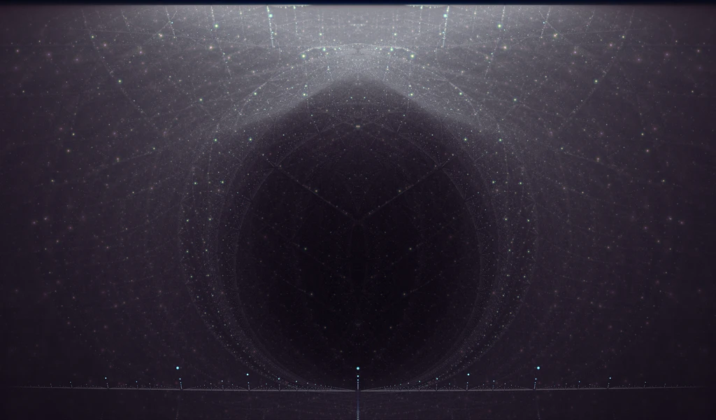
Fibonacci, is that you?
We want to start out as simple as possible which means minimizing the number of proportionality constants. Since the golden ratio provides us only with a single constant (in addition to 1) it is the obvious choice — so we'll shall start by looking into the higher powers of Φ. From before we already know its square is equivalent to a simple sum we can just multiply that sum by Φ, simplify all products into further sums, combine, and be presented with the sum expression of Φ³. For the further powers a simple rinse and repeat will be enough. Even before we see what the actual results are we can already know that it will be always be possible to express the results in terms of simple multiples of 1 and Φ since the square is the only non-trivial product we will come across, and we already know how to dismantle it.

Looking at the resulting columns of coefficients separately we can identify a familiar pattern. The multiples of 1 and the multiples of Φ both follow the Fibonacci sequence in which the next number is always the sum of the two previous ones. This recurrence is a well-known property of the golden ratio. Similarly it is known that the ratio between the two coefficients works an approximation of Φ — the larger the exponent the better that approximation. This actually ties in neatly with the continued fractions introduced in the first post. Recall that Φ is an irrational number which means it can be represented as a unique infinite continued fraction. It is also the simplest one of all of them since its ones all the way down. Let's see what its finite continued fraction approximations look like.

As we mechanically simplify the finite fractions into simple rational numbers (with intermediate steps omitted) we see that they follow the same pattern as the coefficients and thus provide us with the very same approximations. The fact that this very simple pattern manages to manifest itself in these seemingly separate contexts is a testament to its elegance. As a minor side-note, since the coefficients of the continued fraction are all one the approximations converge slower than for any other infinite fraction giving the golden ratio the dubious honor of being the most irrational number.
Although I began the post by talking about multiplication hypercubes and the problems they would pose it turns out that we have actually managed to completely describe this strange exponential product-space for the special case of the golden ratio. Explaining why this is so requires us to use some light geometry, although simply put it is due to the small number of proportionality constants involved. Consider the multiplication table associated with the golden ratio, a simple 2x2 square. Extending it from its quadratic plane into cubic dimensions makes it a 2x2x2 multiplication cube. However, due to the necessities of its construction three of its faces are the same as the multiplication table it is derived from. So, by adding an extra multiplicative dimension we have only added one previously unknown result which is located opposite to 1 at the other end off the (very short) three-dimensional main diagonal of our multiplication cube — Φ³. When we keep adding dimensions corresponding to the higher powers of Φ this linear growth pattern continues despite our initial geometric fears. See the marvelously unintuitive multiplication hypercube diagram below, with the directional axes of the four-dimensional product space highlighted in color. Each line corresponds to either a multiplication or division by Φ depending on the direction of travel.

The multiplication tesseract naturally encloses within itself the entire progression of product spaces — from line to square to cube to hypercube. Can you find the six copies of the multiplication table and the four deformed copies of the multiplication cube? Whenever we add a multiplicative dimension we double the number of results (vertices) with the new values being a simple multiplication (by Φ) of the values of prior lower dimensional vertices. In summary, the simple Fibonacci-like sequences we saw before allow us to easily generate all the possible factorizations found within the multi-dimensional product spaces of the golden ratio. As a direct consequence of the way the higher dimensions are extruded, if we start from 1 and only travel along these extrusion edges we see that the first step away from our origin takes us necessarily to a Φ-vertex. After that, our next step (unless we go back) takes us to a Φ²-vertex, and so forth. Interpreted in this way the exponent of a vertex becomes equal to its Manhattan distance from the origin. Each successive pair of Fibonacci numbers directly gives us the factorized coefficients of the next diagonal product in our geometric progressions.
Powers beyond golden
The question I originally asked myself at this point was: are there Fibonacci-like sequences embedded also in the geometric progressions of the other optimal sections? In hindsight the answer is: of course! We already know their two-dimensional product spaces from the previous post so constructing their higher dimensional equivalents will be straightforward. So let's just calculate some of them out for the smaller constant of the golden trisection.

Not very encouraging yet. There seems to be no Fibonaccis or any other recurrence patterns running down the vertical coefficient stacks. To see what's going on we need to widen our perspective a bit. Abandoning the strictly vertical, one thing that we can easily see is that the first unit coefficient is always equal to the ρ-coefficient of the previous row. This is a straightforward consequence of ρ² expanding out to 1+σ. As we saw in the previous part, the perfect square analogues (ρ² and σ²) which lie on the main diagonals of the associated multiplication tables are the only products whose sum factorizations contain a 1. Since we are always multiplying everything by ρ its square will be the only term that produces 1's for the next product. Hence this direct correlation. This should also give you a hint regarding the recurrence patterns.
As soon as we start looking for cross-column recurrences the other patterns present themselves. Probably the most obvious clue is the two 14's showing up in the factorization of ρ⁷ and then 28 making an appearance on the next row. Prior to the seventh power we can find 9+5 making 14 and for the ninth power we can see that 47 is made up of 28+19. This is again a direct consequence of the binary products and their sum factorizations: ρσ and ρ² are the only products who sum factorizations are defined in terms of σ (corresponding to the middle-column). Similar recurrence relations are also found in the geometric progression of the larger trisectional constant. You can see these recurrences represented visually in the diagram below. They are not as neat and tidy as the simple Fibonacci associated with the golden ratio, but they are definitely something!

Figure 2: Connectomes
Note the slight difference in the ordering of terms for the two different trisectional progressions. The structural pattern of the recurrences is of course independent of the term order we choose, but choose we must if we wish to compact the results into pure number-sequences similar to the original Fibonacci. Luckily, due to the limited number of constants there aren't that many viable options. If we use the powers of Φ and their embedded Fibonacci sequence as a starting point we can see that a kind of deduplication is necessary to recover the unaltered sequence when reading out coefficients row by row. For the purposes of the number-sequence construction the two directly correlated coefficients (connected in red) are considered to be the same number. We naturally assume that this same deduplication should apply to the other sequences we construct.
This direct correlation gives us a very straightforward way to "glue" the individual rows of coefficients together and for it to be possible without awkward overlaps the two directly correlated numbers must necessarily be the last and first terms in the ordered sum factorizations. In other words, due to the perfect square property discussed earlier, the unit constant 1 should always be the first term and the chosen multiplier should always be the last. Happily, this leaves only one possible place for the last unpositioned term. Now, obviously this only works for the trisection which means that we will have to find a more general approach as soon as we start to consider the other n-sections. In any case, let's see what the number sequences look like when we glue them together.

In case you didn't already guess it from the blue-colored connections of Figure 2, the trisectional sequences do in fact contain the basic Fibonacci recurrence. It was difficult to notice only because it was interleaved with another recurrence pattern. In the case of the ρ-sequence the other recurrence is a kind of delayed Fibonacci where the sum is produced not from the two previous numbers, but from the two numbers before those. The additional recurrence relation of the σ-sequence on the other hand is sort of delayed Fibonacci involving three numbers (Tribonacci, anyone?). For completeness, the recurrences we previously visualized as colored line-connections are now stated in their mathematical form below. For the time being, everything that comes before the start of the displayed sequences (n=1) can be considered to be zero.

However, this is as far as we get with the sequences generated so far. So the next obvious step is to produce the comparable sequences for the other optimal sections (beyond golden) and see if there are more interesting patterns for us to find. Note that we can already deduce the kinds of recurrence relations we are going to find in the sequences simply by looking at the multiplication tables of the previous post. If we choose a column corresponding to the constant we are multiplying by, then on each row of that column the number of terms corresponds to one of the interleaved recurrence relations of the coefficient sequence – or symmetrically for row and columns – with the first row/column corresponding to the direct correlation we chose to compact earlier. Although the details of indexing will depend on the term order we end up choosing we can already predict that the coefficients of α will be the consequence of three Fibonacci-like two-term recurrences. In fact, since the second column (or row) is always composed of at most two terms we know that all coefficient sequences of all Ψ₂ will be the result of recurrences which involve only two previous values (at further and further distances). What slightly complicates things is that the total number of such interleaved recurrences grows linearly with the number of proportionality constants.
Order from chaos
As we now begin considering the coefficient sequences of the more numerous optimal sections we are properly confronted with the problem of term ordering. Our fledgling first step was to assert that in order to avoid coefficient overlaps the constant term (multiples of 1) should always be the first/leftmost one and that the multiplier (whose geometric progression we are considering) should be its counterpart, the last/rightmost term. This we justified based on their unique correlation made necessary by the oneness property of the perfect squares. As we deduced in the previous post, the perfect squares of the proportionality constants that form the main diagonals of the associated multiplication tables are the only products whose sum factorizations contain a 1-term. Our assertion gives us only two positions which leaves the open question of: what is the right way to order the terms in the middle? Or in the absence of a right way — is there a way to order the sequences so that we can see if there are any similarities to be found?
Sequence-wise, no such similarities were to be seen in the the sequences we saw earlier although they did exhibit some similarity in terms of their defining recurrence relations. Comparing the geometric progressions of the smallest non-one proportionality constants of different n-sections (Ψ₂, also known as Φ, ρ, α, and θ) offers us a convenient direction of investigation. Under recursive multiplication their smaller numerical values translate to fewer terms with smaller coefficients. In the absence of known rules, let us for the time being order the terms the same way we ordered the proportional line segments in the previous post. It neatly matches our partial description for the orderings of Ψ₂-sequences: leftmost term being 1 and the rightmost term being Ψ₂, with the middle filled in left-to-right first with the odd-indexed constants and then with the even-indexed constants in reverse order. Let's start with the optimal quadrisection's α constant.

Figure 3: Connectome of α
Again the recurrence relations are visualized as colored line connectors from which we can verify our earlier extrapolation that the coefficient sequence of α contains three Fibonacci recurrences (one normal, two delayed). As a happy little accident the sum of the connecting lines resembles the polygon that gives rise to the involved proportional constants. Recall the polygon-section relation k=2N+1 we derived in the first post — the nonagon (k=9) is the associated polygon of the optimal quadrisection (N=4) to which the proportionality constant α relates to. With a little applied imagination (what is the missing ninth point?) we can draw a nice geometric diagram which visualizes the rules of α-multiplication. Looking back, we can see that there are similar unwound polygons hidden within the recurrence relations of ρ and Φ as well.
Also as we suspected, the small value of α in relation to the other constants causes the geometric progression to get into full swing only after the fifth power. Unfortunately, this leaves a lot of empty spaces which correspond to an equal number of zeroes in the generated number sequences. Leaving them out as a simplification is more expedient for the purposes of sequence comparisons although doing so does mean obscuring the embedded recurrence relations. But, we can ignore them for now, especially since they do get rather involved. Let's see what the various coefficient sequences look like without their zeroes.

It seems that our placeholder ordering proved to be the right choice. The ordinary Fibonacci turns out to be the exception rather than the rule and fairly quickly the visible portion starts to converge, becoming completely identical in the case of the 6-section and 7-section constants (at least for the part shown). The pattern also holds seemingly for all higher sections — the finer we cut the longer the stretches of similarity become. Producing the comparable sequence for the optimal 10-section gives us the first ninety stable numbers of this sequence. Although this sequence of numbers seems to be of some significance in our context it is not included in the Online Encyclopedia of Integer Sequences (or OEIS). This is a fairly good indication that this sequence is not too important, at least not on its own or in this particular form.
Another problem is that we did not manage to learn much about the term ordering. Our initial guess was a fortunate one, but we can apply that order only to these generalized Fibonacci sequences. Beyond them, our multiplier changes and with it, so must the rightmost term. With some effort we can calculate a bunch of geometric progressions for various proportionality constants, initially sequencing their terms based on some arbitrary (but consistent) order, and then attempt to line up their identical runs in the hopes of some regularity in the ordering. The sequences of the larger constants do in fact result in similar sequence stabilization events although the stable portions converge much slower than Fibonaccis relatives. Fortunately it is fairly straightforward to produce these sequences and run the comparisons automatically (with the help of a small program) saving us a lot of manual work. You can find some of the stable prefixes of the generalized sequences below, with the sequence sub-index indicating which proportionality constant it corresponds to. For example, F₃ is associated with σ, β, κ and more generally all Ψ₃.

Although all of the sequences curiously stabilize out of initial noise none of them seem of any consequence as far as the OEIS is concerned. Also, aside from some recurrence pattern similarities the sequences of different index seem to share no other resemblance. The converging sequences arising from proportionality constants that share the same ordinal index is still encouraging though, so all is not lost! Figuring out these sequences allows us to formulate (with considerable effort and some luck) a rather straightforward ordering rule that generalizes for any constant of any optimal section. This permutative pattern is perhaps best explained with a visual aid.

Figure 4: Term-order permutations
The first term order correponds to the proportional line segment ordering mentioned earlier. To derive the next term ordering we take all the terms except the leading one and reverse their order leaving Ψ₃ as the rightmost term (as desired). Then, to derive the next ordering we now ignore the first two established terms and reverse the order of the remaining ones. We keep going in this fashion, always adding one more term to the immutable prefix (underlined in blue) and reversing the rest (enclosed in square brackets). Following this permutative pattern to its conclusion, the last ordering we get has all the terms in perfectly sequential order. Using this seemingly arbitrary, but rather elegant strategy we can find the comparable term orderings for all possible geometric progressions derived from the optimal sections. This mechanical rule works regardless of the total number of terms involved, so even if this isn't the absolute right order at least it's highly practical!
If you liked the geometric visualization of the α-multiplication you might also like these which we can now construct based on our formulaic term orderings. In the context of these visualizations the orderings are perhaps less decisive, but at least the first and last polygons of each set do seem particularly elegant. It is also not obvious to me why they should end up being so symmetric, but it certainly adds to their visual appeal. This concludes our investigation into the geometric forward progressions of the proportionality constants, although we will return to their embedded sequences in the next post. With the higher powers taken care of, we could ask the question that got this whole series started: what about the negative exponents?
Lower powers
This is where things get decidedly harder. The maximal optimality of our proportional sections guaranteed that we would be able to decompose all possible multiplicative products into equivalent sum expressions. It made no such guarantees about the inverses of the proportionality constants. Furthermore, to begin the construction of the constants and their multiplication tables we relied on a spark which seemed to be irreducibly trigonometric in nature — remember 2cos(π/k)? I can think of no reason why its inverse should be easily factorizable. From the numerical magnitudes of the constants we can deduce that at least the inverses cannot be pure sum expressions. There must be some subtractions for the values to end up being less than one. However, if you remember we did actually stumble upon some inversional examples in the first post of this series. There is of course the familiar golden ratio inverse (1/Φ) which we know to be equal to Φ-1. The other inverse reinterpretations we found through simple trial and effort were 1/ρ = ρ-σ+1 and 1/σ = σ-ρ (from which σ/ρ = σ-1 and ρ/σ = ρ-1 can be derived).
Again, to start simple let's look at how the inverse of the golden ratio can be derived. Consider its known equivalence statement Φ² = 1+Φ. When we wanted to find the third power all we had to do was multiply both sides by Φ and then decompose all multiplicative products into their known sum expressions. Whatever was left on the right side of the equation was our answer. Nothing prevents us from trying to go the other way by dividing both sides of the equation by Φ. In at least a few particular cases we know that there must be way to similarly simplify the equations into equivalent addition/subtraction combinations.

All well and good. We should be able to do the same for ρ and σ. Although remember, that the multiplication tables grow quadratically which means that for the optimal trisection we will need to apply our divide and conquer strategy to up to four equations. We can get by with less if considering things in isolation does the trick (which it doesn't), but with a little more effort than before we manage to figure things out nicely — easy to stay motivated when you know there must be a way. Notice how we first need to figure out the comparative ratios of ρ and σ before we can solve for their inverses.

You can probably see why solving the inverses in this manner quickly becomes problematic. The next optimal section would have us solve nine similar equations, and the one after that would require sixteen. There seems to be no shortcuts either as the solution of the simple inverses is predicated on solving the other ratios first. The bad news is that there seems to be no way around this quadratic growth of our problem space. One way or another the solutions are going to be taking a lot more time for larger optimal sections. As a small comfort there is at least an equivalent, but slightly more streamlined way of finding the inverse factorizations. We begin by knowing that something multiplied by its inverse is one and then assuming that the inverse can be represented as a simple factorization.

Once we have regrouped the AB-coefficients into a more suitable arrangement we can see straight away that for the equivalence to hold true B must be one and A+B must be zero (since there are no Φ's on the right side of the equation). This allows us to trivially deduce that A must be minus one, which concludes the solving process. At first this may seem like more work than the earlier method, but it does have its upsides. First, we can already extrapolate that whatever the final simplified form of the equivalence happens to be all the individual coefficient sums must be either one or zero — all the coefficient-sums that act as multipliers of non-unit constants must be zero since the right side of the equation contains none of those (A+B in the above example) leaving only the unit constant coefficient which must be equal to one (B in the above example). Second, there is a pretty easy way we can find the desired arrangement of coefficients simply by utilizing the multiplication tables allowing us to entirely skip the tedious term shuffling. Let's see how it works for the heptagonal inverses.

First we label the columns of the multiplication table with the coefficient symbols we wish to use. Then, to find the equivalence that allows us to solve the inverse corresponding to a row (first row corresponding with the inverse of one) we proceed by asking a series of questions. First, in which columns does 1 make an appearance? Due to the previously discussed property of perfect squares we already know that it will only make an appearance along the main diagonal. So for each row, there will only be one column that includes it. The label of that column will give us our constant coefficient (multiplier of one) for the associated equivalence statement.
Next, in which columns does ρ make an apperance? For the first row it appears only in the column corresponding to B, but in the case of the second and third row ρ makes and appearance in two columns — resulting in the coefficient sums A+C and B+C respectively. Finally, in which columns does σ make an appearance? Again, first row is trivial. On the second row there are two relevant columns (B and C) while on the third row all columns contain a σ. In this manner we can easily construct the coefficient sums of all the related equivalence statements. Following the same logic as before we attempt find concrete solutions for these coefficient sum constraints. Figuring out the solutions allows us to reconstruct the assumed inverse factorizations.

In the case of the first equivalence the solution is trivial and with fairly little effort the constraints of ρ and σ are also solved (especially since we already know the answers). Since we know how to construct multiplication tables for arbitrary optimal sections we can also easily derive the associated equivalence statements. The only real problem in finding the inverse factorizations is solving the resulting coefficient constraints. Although even that turns out to be a fairly straightforward matter, but I won't go into the details here. Really, the only practical limitation is the growth-rate of our problem space. The total number of constraints is always equal to the number of constants (with 1 included) and the maximum number of coefficients in each constraint is also equal to the number of constants. Both grow linearly which means their combination – the total number of coefficients in our set of constraints – grows quadratically. Not great, but also not terrible.
The unfactorizables
Unfortunately, when we try to apply this method to the next optimal section we run into a problem. Although our method of construction for the equivalence statements and the resulting constraint sets works just fine one of the constraint sets turns out to be not only unsolvable, but contradictory. This means that our initial assumption about the straightforward factorizability of the associated inverse is incorrect. Consider the following equivalence statements and the constraint sets of the optimal quadrisection constants – α, β, and γ.

The constraints of α and γ have fairly straightforward solutions. In the case of α, the solutions cascade nicely — B gives us D, which gives us C, which gives A. Plugging the coefficient solutions into the inverse factorization we assumed for α makes it equal to -1+α+β-γ. For γ, a similar cascading takes place although we can also take a kind of shortcut by utilizing the constraints themselves to facilitate the solving process. Knowing that C+D and B+C+D are both equal to zero implies that B must be zero. In a similar way, knowing that B+C+D and A+B+C+D are equal to zero implies that A must be equal to zero. Whether we use the shortcut or not, the value of C is solved trivially by knowing D. In any case, the inverse of γ is seen to be equal to γ-β.
So far so good, but for β the constraints present a contradiction. Knowing that C is equal to one and that B+C+D is equal to zero allows us to deduce that B+D must be equal to minus one. However, one of the initial constraints states that B+D is equal to zero. Obviously, both cannot be true at the same time, and yet both are seemingly inevitable conclusions. Even without this contradiction the set of constraints would offer us no way to solve further (unless we resorted to guesswork). Due to the relatively low number of terms involved we can verify this unfactorizability with a simple brute force search and attempt to exhaustively guess our way to a solution — never finding any. There's just something special about β.
As we solve for more inverses we find that the next optimal section (of θ, κ, λ, and μ) is completely solvable. As is the next one after it. Then however, the optimal seven-section corresponding to a fifteen-vertex pentadecagon offers three solvable inverses and three contradictions. The next two optimal sections after that contain only solvable inverses, but then for the optimal ten-section corresponding to a twenty-one-vertex polygon there are four contradictions together with five solutions. Accumulating ever more samples several patterns start to become apparent. The two most obvious ones relate to the nature of the smallest and largest inverses within each proportional number system. First, they seem to always have factorizable inverses. Second, we don't really even need the solving step to know their factorizations and you can probably see why.

Largest constants = smallest inverses

Smallest constants = largest inverses
The inverses of the largest proportionality constants are all just simple two term subtractions — largest minus the second largest. Almost boringly simple. However, the factorization patterns of the smallest proportionality constants more than make up for that. They are always the most complicated inverses within a given number system as they involve all the available terms. A neat ordering can be established which reveals the alternating sign patterns interleaved between the ascending even-indexed constants followed by the descending odd-indexed constants. Note how the ordering is the exact reverse of the order we chose for the geometric forward progression of the same constants. For that same reason, if you read the second post in this series it should also seem visually familiar to you.
The patterns in the above inverse factorizations are a direct consequence of the associated multiplicative product factorizations, as revealed by our solving method. The second column products (of the smallest constant) are always sums of two terms whose maximally interleaved ordering guarantees the widening patterns in the corresponding inverse factorizations. In the case of the largest constant the relatively straightforward triangular pattern of the multiplicative factorizations results in most of the coefficients resolving to invisible zeroes. However, as already hinted at by the unfactorizable inverses, between these two monuments of regularity lies a rather more uneven landscape. One thing we recognize about the factorizables inbetween is that their signs are always as balanced as possible — meaning that the difference between the total number of positive and negative signs is at most one, and always zero if the factorization has an even number of terms. This same pattern also applies to the regular factorizations we saw earlier. Perhaps the most important (and also the most obvious) pattern in the inverse factorizations echoes their multiplicative relatives: all the multipliers are either plus or minus one!
Aside from the patterns pertaining to the inverse factorizations there's also the question of the unfactorizables. With enough samples they also start to exhibit a pattern of their own which I think is even more fascinating than the one regarding the factorizables. Recall that so far we have seen contradictions arise for optimal section polygons with 9, 15, and 21 vertices. The next unsolvables after those are found for polygons of 25, 27, and 33 vertices. Due to the section-polygon relation (k=2N+1) we know that the even polygons do not relate to our current context, so they are absent by definition. The pattern is perhaps most obvious if we list the polygons corresponding to the fully factorizable inverses: 3, 5, 7, 11, 13, 17, 19, 23, 29, 31. Looks an awful lot like prime numbers! And funnily enough, the unfactorizability of inverses seems to correspond to a factorizability pattern of another kind. In the list below k corresponds to the number of vertices in the associated polygon (remember that Ψ₂ = 2cos(π/k)) and N corresponds to the degree of the optimal section (and thus also the maximum constant index).

Whenever k is divisible by some number then the constant indices corresponding to multiples of that number do not have factorizable inverses — a factorizable k makes for unfactorizable 1/Ψ's! Just to give an example from the table above, since the ten constants of an optimal ten-section are related to a twenty-one-vertex polygon, and because twenty-one is divisible by three and seven, the proportionality constants three, six, seven, and nine do not have factorizable inverses. This pattern seems to hold true for as far as I have been able to verify, and the sixty-seventh proportionality constant of the optimal hundred-section (Ψ₁₀₀,₆₇) does not have a factorizable inverse because the associated 201-vertex polygon is divisible by sixty-seven, while at the same time the inverse of the second constant of the same set can be factorized by using a total of a hundred terms! I have absolutely no idea what strange logic gives rise to this remarkable property. How can there be such a link between the factorizability of one thing and the non-factorizability another? Why are the prime-numbered optimal sections somehow more complete and symmetric than the non-primes?
Sequence symmetry
Equipped with this newfound knowledge we can (almost) arbitrarily produce factorizations for the inverses of proportionality constants, and once we know the inverse representations we can simply keep recursively multiplying and simplifying (like with the forward progressions) to get the factorizations for exponent of minus two and beyond. We can do this at least for all "prime constants" for which an inverse factorization can be found. This opens the door for us to start considering their inverse geometric progressions and the coefficient sequences that run along them.
In the next part we will do exactly that in the context of a wider investigation of the ► Embedded Sequences. Can you already guess how they relate to quantum spin physics?