


C2. Optimal sections
In the previous part we dipped our toes into the weird dynamics found in iterated continued fraction functions. If you haven't already I highly recommend checking it out before continuing with this part. It introduces our initial set of proportionality constants related to the golden ratio. It also describes in detail the fractal framework in which these constants play an important role. As mentioned in that previous part, the straightforward geometric construction with which these constants can be derived is something I figured out only afterwards. Although the geometric construction is elegant in its own right, wrapping everything up in geometric language makes it easier to miss the strange algebraic properties that these proportionality constants possess.
When I was first trying to figure out the continued fraction gap structures I derived the values for the constants from their proportional relations. Out of the initial set of previously studied optimal sections and their known proportions I managed to figure out some generalized patterns that allowed the construction of further sets of constants and their optimal relations with relative ease (no pun intended). At that point things started getting weirdly interesting.
Although this time we don't have a strict need for a reference image as far as the explanations go I'd still like to start things off with one of the images that got this enjoyable rabbit hole started. The proportionality constants we are going to be exploring also give rise to the fractal dynamics you see in the image.

The multiplicative alternative
My original search for the meaning behind the seemingly arbitrary numbers associated with the fraction gaps originally lead me to this page discussing the golden trisection — a three-way relative of the golden ratio which I had never heard of before. It showed how the proportionality constants related to the seven-sided heptagon could be derived via geometric means. My geometric skills being what they were (and still are) I wasn't too keen on extrapolating these constructions out for arbitrary polygons, although in hindsight it turned out to be pretty straightforward. However, at the time I just skimmed the page for the parts that seemed most relevant for my immediate purposes. Most helpfully it listed as one of it references a paper called Sections Beyond Golden by Peter Steinbach.
The paper studies in some detail the various aspects of the golden ratio and trisection, and it also briefly shows the optimal quadrisection and pentasection. Without his fortuituous – and according to him, somewhat accidental – discovery of the three optimal sections beyond golden I probably would never have figured out the pattern of the continued fraction gaps, so thanks Peter! What proved particularly useful was a diagram depicting the four polygons related to the four optimal sections, the diagonals associated with the proportinality constants, and the proportional relationships between the constants. The image below is a reproduction of the figure number #5 from the original paper (a casual death metal reference). It is the skeleton key from which everything follows.

The relational language shown in its original form is perhaps a bit difficult to parse if you are previously unfamiliar with it. The letter pairs correspond to various line segments whose lengths are equal to some additive combination of the associated constants. In the case of the pentagon (golden ratio) the proportional relation can be expressed more verbosely as follows: the smaller part (AB) is to the larger (BC) as the larger part (BC) is to the whole (AC). Personally, I find the equivalent mathematical statement to be the easiest to grasp: BC/AB = AC/BC = Φ. Unfortunately, whichever formulation you pick they all become rather unwieldy for the heptagon and beyond. Luckily there is a somewhat easier way to grapple with this abundance of proportions. In fact, we only need to apply some first grade math to find a more compact representation. You might have heard of multiplication tables before.

A table like this makes figuring out the result of a multiplication a simple lookup: pick a column and row corresponding to the multiplication you are after and find the result at their intersection. Since multiplication is commutative (4x2 = 2x4) the table is symmetric with respect to the main diagonal. This diagonal symmetry-axis contains the perfect squares which are all a result of multiplying some number by itself (eg. 1, 4, 9, 16, 25, and so on). The diagonal symmetry means that the upper right triangle of the multiplication table is a diagonal reflection of the lower left triangle. Pretty straightforward, but what's this got to do with us?
Take another look at the blocks of "AB-to-BC" proportion relations in the earlier diagram. They also exhibit a similar kind of symmetry with respect to their main diagonals. The first row and column correspond to singular line segments which represent the proportionality constants themselves. The thought of multiplying line segments together might be a bit unintuitive so in the interest of simplification let us rewrite these relations in terms of the symbolic constants. Can you see the resemblance now?

Although there is an apparent resemblance, there are also some differences. Firstly, in the absence of an infinite set of numerical symbols these tables actually end and offer no obvious way for extending them beyond their individual fixed size. Secondly, the multiplicative results are always expressed as sums of two or more constants, with 1 making an appearance only along the diagonals. With the exception of the golden ratio (equal to (1+√5)/2) this is indeed the only way the results can be expressed without resorting to approximations or arithmetic monstrosities such as these. This is a rather remarkable property when you think about it! Within these finite proportional number systems all these multiplicative combinations can be re-expressed as simple additions with all of the resulting sums only using constants belonging to the originating set. All this without any of the individual results ever needing to use the same constant twice.
Looking closer we can identify even more patterns. The first row and column necessarily use only singular terms since something multiplied by one is by definition that thing in itself, but with those unit results excluded all multiplications involving the first proportionality constant are expressed as sums involving exactly two terms. Then, all multiplications involving the second constant (but not the first) are expressed as sums involving exactly three terms. Further, all multiplications involving the third constant (but not the first and second) are expressed as sums involving exactly four terms. So on and so forth, with each subset forming an L-shaped table cutout rooted in the main diagonal. The square of the largest constant in each set serves as a kind of cherry at the bottom right corner: its square is always equal to the sum of all the constants, including the unit constant 1.
The property that I personally consider the strangest of all is also perhaps the easiest to miss. No matter how many terms the multiplicative results have they will always be adjacent to one another on the end-to-end line segment spans shown earlier. Of course, this is necessarily how the ordering must work if you want to write down the proportional relations in terms of the line segments, like Steinbach did. However, there is only one way that the terms of the various optimal sections can be ordered if one wants to end up with this curious continuity. The fact that such a perfectly measured and unique order should even exist is not obvious to me — why don't 1+λ or κ+λ+θ make an apperance in the solution space? In the paper these non-obvious, but absolutely essential, orderings were arrived at only by a process of elimination. This approach does not scale for our purposes since the number of possible orderings grows in relation to the factorial of N — we would quickly run out of patience. The example below should illustrate this just-so convenience. More on the problem of term ordering in the third part of this series.

Armed with these elegantly self-contained multiplication tables it is possible with some light algebraic manipulations to derive the values of the constants in terms of each other. Which also means that I kind of lied when I said that this would be a non-geometric construction as we still need to figure out one constant (preferably the first) using the geometric means detailed in the previous post, but from there on onwards the rest will follow. Luckily, the first proportionality constant of each optimal N-section is equal to the shortest diagonal of the associated polygon of k vertices with the section-polygon relation given by k = 2N+1. For example, the golden trisection (N=3) is associated with the heptagon (k=7). With very minimal trigonometry (which I will not repeat here) it is possible to figure out that the lengths of these shortest diagonals work out to be equal to 2cos(π/k). To get started with the light algebra let us restate the results given by our multiplication tables in a more suitable form.

It is perhaps a bit non-obvious at first, but these equivalences can be made to work as a sort of ladder that allows us to produce the values of the other constants one-by-one as long as we know the value of the first one — our first rung on the ladder. The next step is the only one we can take: derive the value of the second constant by using the first. Once we climb higher on this ladder it becomes possible to derive the further constants in multiple different ways (all of which are equally valid). The simplest of these derivations always correspond to the second column (or symmetrically, second row) of the original multiplication tables. Since those results consist of only two terms they leave us with fewer terms to consider on the right sides of our equations. Below, I've chosen to include just those simplest derivations. The other ones aren't too complicated either as long as the number of terms remains relatively small.

This route allows us to almost entirely side-step the trigonometry making it possible to calculate the values of the larger constants with just some light multiplication and addition. However, despite our sleight of hand the true underlying nature of the constants would certainly seem to remain primarily geometric.
Going beyonder
Okay cool, so what next? Steinbach's paper nor any other source that I could find goes beyond this point. This means we are on our own and it is pretty easy to understand why. In the end these "sections beyond golden" are rather niche curiosities with limited practical applications. Indeed, aside from art and aesthetics no obvious applications come immediately to mind. So it is possible that no one has simply had any motivation to look further. However, since the optimal sections turned out to play such a key role in the gap dynamics of continued fraction fractals I was determined to take things as far as they would go.
At this point – due to the limited size of the Greek alphabet – I decided that I needed a new notation that could be more easily extended. I somewhat arbitrarily decided to use the greek letter psi (Ψ) and combined it with a pair of sub-indices to denote the associated N-section (first index) and the sequential number of the proportionality constant (second index). For reasons that will become apparent only later I chose to assign the sequence number 2 to what I have so far been referring to as the first proportionality constant (I apologize for this potential confusion). Instead, the first sequence number is henceforth associated with the unit value of 1 for all N. On that same note, whenever the primary index can be deduced from the context I will leave it out in favor of reduced visual clutter. Applying this new convention retroactively to Φ and to the symbols used by Steinbach hopefully makes the new notation sufficiently clear.

So, if we want to keep the amount of trigonometry to a minimum how should we proceed for the N=6 constants? If we completely ignore the alternative trigonometric solution we also have no foreknowledge of the proportional relations beyond the pentasection. All we really have are a few examples that may or may behave according to some grander patterns. Naturally, since I am writing this post exactly such a pattern can be found.
As per our earlier derivations the value of the second constant seems to always be equal to the square of the first one minus one. At least almost always. It cannot be the case for the golden ratio since there is no second constant. The absence of the second constant handles itself rather elegantly though: the square of golden ratio minus one is equal to the golden ratio itself! Drawing overly sure conclusions based on our small sample size we assume it to represent the only exception to what is otherwise the rule. Unfortunately, such a small leap gives us only one of the results in a multiplication table with fifteen unknowns. What's worse, the number of unknowns grows quadratically with N. So instead of working out things on a per-constant basis in this way, what we really need to do is figure out the overarching patterns in the multiplication tables themselves. Finding and learning these patterns would allow us to construct bigger tables at will. Let us apply our new notation to the first two columns of the multiplication tables we've seen so far. Primary indices of the second column are omitted so as to put more emphasis on the sequential indices.

If we consider the left and right-side terms within the second column separately and look at their respective sequential indices a fledgling vertical pattern presents itself. The left-side sum operand indices, starting from one, follow it perfectly. The right-side, starting from two, shows a minor hiccup though. If it followed a similar linear pattern the last index would go outside the range of definition: what is the sixth constant in a number system consisting of just five constants? Generalizing the exception we saw in the case of the golden ratio we make an assumption that in the absence of a "next" constant the last constant simply loops in on itself. In other words, the index increment is simply skipped for the last row's right-side term. While not exactly elegant, it's has some potential. Especially since the first two columns are all we would really need to be able to reproduce the proportionality constant values of arbitrary N-sections. In fact, if our immediate goal is simply to determine these values we don't even need the annoyingly exceptional last row. So if our guess regarding the indexing pattern of the second column sum-terms is correct it offers us a way to easily calculate the values of the larger proportionality constants for any optimal N-section without involving any trigonometry! In mathematical language we can express the recurrence pattern as shown below — the ghost of Pafnuty Chebyshev has returned to haunt us. The derived proportionality constant values for the optimal hexasection (N=6) are also included. They are equivalent to the diagonals of a thirteen-vertex tridecagon.

However, these numbers in themselves are meaningless unless their interrelations do not give rise to optimal sections similar to the ones studied by Steinbach. Up until now we haven't really even defined what optimal means in this context. So suppose that instead of using the values derived above we picked some other five numbers. If we then tried to construct similar "AB-to-BC" relation blocks and realized that some relational lengths could not be expressed as combinations of existing line segments it would mean that we were left with fewer relative proportions. For the equivalent multiplication table it would mean that some results in the table were simply arbitrary numbers rather than neat sums of existing terms. This would make those five numbers a less optimal sectioning with fewer interrelational proportions than those we've seen so far. Indeed, the fact that the multiplication tables are fully populated with neat sums means they are as optimal as possible! These properties can also be understood in the context of multi-parameter function systems which interestingly enough give rise to negative proportionality constant solutions which produce equally maximal optimal sections! I won't go into that here though.
So really, in order to prove the optimality of the hexasection constants we produced earlier we need to fill in the rest of the multiplication table. Which means we need to figure out the patterns for all the columns and all the rows. Lucky for us, the pattern we found in the second column has analogues in the third column and beyond. Instead of going them through one by one I will simply show the conclusions I drew and how they can be applied to the multiplication table of the hexasection. Because of the unwieldy horizontal girth of the complete multiplication table I've chosen to include only the last column where the overarching pattern is most obvious.

Click to see full table
The apparent awkwardness of the second column's index-pattern reveals its elegance in this wider context. Forget the vertical patterns. Instead, if we focus our attention on the diagonals that run from bottom left to top right (highlighted in red) we can see that within these diagonals the term indexing is entirely sequential. The table would certainly seem to fit the visual description of an optimal section — last square is sum of all constants, one-terms appear only on the main diagonal, and the total number of terms follows the L-shaped pattern described earlier. More importantly though, when verified numerically the multiplication table proves out to be internally consistent. Which offers us sufficient proof that the six proportionality constants we derived earlier indeed do correspond to a maximally optimal hexasectioning.
Extrapolating these patterns of construction out to an optimal section of N=500 and verifying the results numerically they all work out wonderfully — the relative error between the numerically calculated square of Ψ₅₀₀ and the sum of all five hundred terms is only slightly above one trillionth which is good enough for me. Some error is to be expected due to limited floating-point precision. This means we have (at least in practical terms) found the way to construct optimal sections for any number of cuts. I won't bore you with the mind-numbing multiplication tables this involves, but rather I wish to show what kind of line segment orderings are associated with the tables we can now construct freely.
Although we made no explicit effort to preserve the property of term-adjacency, by working backwards from the multiplication tables it is possible to figure out the end-to-end line segment ordering that must necessarily correspond with its sum expressions. The diagram below shows the first seven which are hopefully enough to reveal the underlying pattern further highlighted by the "sweeping areas" formed by the proportional segments.

Stepping through the various sectionings we see that the new proportionality constants are always inserted into the middle. First, from left to right, all the odd-indexed constants are laid out sequentially and joining them in the middle, from right to left, all the even-indexed constants. This curious ordering seems to be the only way to provide the term-adjacency guarantees we wish to maintain (which implies solvable function systems). This would seem to finally exhaust our avenues of investigation, but instead of wrapping things up I invite you to consider what happens when we try to do an optimal infinisection. How can you divide something infinite into an infinite number of unequal pieces so that the total number of proportional interrelations is maximized?
Apeirogon
Meet the extraordinary polygon corresponding to this rather absurd generalization: the mother of all polygons, the infinite-sided apeirogon. Although at first it would seem not to be a polygon at all, but rather a simple line dividing the two-dimensional Euclidean plane into its interior and exterior, it turns out to work just like any other polygon as far as our formulations go. Again, we calculate the first non-one unit constant using the same 2cos(π/k) formula as before. Then we keep mechanically applying the recurrence relation we derived earlier. First time I did this, I was rather taken aback by the results. Also, why I chose the indexing I did should now begin to make sense.

Neatly enough you can just drop the Ψ's and perform the multiplications and additions directly on the sequence indices as the proportionality constants of the infinisection are equivalent to the natural numbers! In the geometric interpretation the natural numbers correspond to the degenerate "diagonals" of the straight-line apeirogon. Needless to say, this worked out much better than I could ever have expected. When we apply our rules of construction and produce the associated infinite multiplication table we realize we have come full circle. Although the simple results of our initial multiplication table have become factorized into sums following the distinctive patterns of optimal sections.

All of these factorized sums are of course equivalent with the natural numbers that the sums represent. Unlike in the case of the finite optimal sections these composite numbers will always be part of our infinite set of proportionality constants further increasing the abundance of proportions. The sum factorizations and their extrapolations allow us to conclude some unconventional and rather non-sensical equivalences found at the infinite edges of our multiplication table. Since the geometric construction method based on sine ratios breaks down completely for the infinisection the equivalences below should not be taken too seriously though. While the first two might seem somehow feasible, the last equivalence should unequivocally tell you that near infinity the numbers have ceased to function normally and we'd best be turning back.

Although it is not clear from the partial multiplication table shown earlier, the behavior change in the vertical index patterns (which is the main culprit for this breakdown in numerical logic) always happens beyond the antidiagonal of the multiplication table — running from lower left to upper right. Everything directly on or to the top-left of the antidiagonal is perfectly uniform and well-behaved, but beyond it the awkward increment skips from earlier return with a vengeance. Past the antidiagonal boundary the sum expressions will start to depend on the size of the chosen number system giving us the weirdness at infinity.
Sticking to the well-behaved parts we can conclude that although the numerical values of the constants may differ for different N, the square of Ψ₃ will be equal to Ψ₁+Ψ₃+Ψ₅ within almost all such proportional number systems. The similar-to symbol in the formulas below is meant to indicate that the sequential indices of the product sum expressions are the same as long as the attached predicate is true. Although the products/sums cannot be equal in value (since the numerical constants are different) they start to converge quickly as N grows. Some explicit examples of the sum-similarities relating to the squares of constants are also shown.

Before we leave this reductio ad absurdum behind us there's just one more thing that is worth visualizing and that is the infinisectional line segment ordering that guarantees the term-adjacency for all the sum expressions found in our infinite multiplication table. For obvious reasons the segment lengths can no longer be represented to scale and in order to compactify the diagram the line segments are wrapped onto a hyperbolic circle perimeter. The implication of this circular construction being that all multiplications can be represented as the combination of a certain number of adjacent sectors (that don't span zero). The prime numbers which famously don't factorize in terms of multiplications are the only numbers which have a singularly unique representation in terms of these adjacency sums — they are the only self-defining numbers.

Similar circle sector constructions for few of the first finite sections can be seen here this time with angle proportions preserved (and with colors corresponding to the previously shown diagrams). Also, remember those faint branching structures related to the continued fraction gaps that also show up within the Mandelbrot set? They look awfully similar to the branching structures found in the order-3 apeirogonal tiling of the hyperbolic plane.
Higher powers?
Due to the two-dimensional nature of the multiplication tables we have constrained ourselves to multiplying only two numbers together (a binary product). In geometric terms we only looked into squares and rectangles. The obvious question is: what about cubes and cuboids? A ternary product which multiplies three numbers together would correspond to these three-dimensional shapes or rather, volumes, but if we were to continue with our previous methods this would require us to deal with corresponding multiplication cubes! Unfortunately, they aren't quite as practical in human-terms as flat tables and what's worse, a four-product and a generalized n-product continue the trend into higher-dimensional hyperrectangles. Multiplication hypercubes? Forget about it. However, there is one way we can use to at least partially investigate these structures while still preserving our sanity.
In the next part of this series we will investigate the geometric power progressions of the various proportionality constants. The ► Higher Powers of these constants (as well as their inverses) give rise rather curious new patterns, taking us deeper within our present rabbit hole.