202. Centerpieces

The Outside

There are many different ways to visualize the Mandelbrot set, but arguably the simplest and most widespread is the "escape time" coloring algorithm — where the time being measured is the number of iterations until a sequence escapes (ie. diverges) to infinity. This is the same approach that we used in the demo of the previous post. Recall that by definition no point within the Mandelbrot set ever diverges which means that the interior points cannot be assigned colors in this way. Instead, they are usually colored black. For this reason it would be more accurate to say that the escape time algorithm is drawing the outside of the Mandelbrot set.

Since the numbers can never become truly infinite in finite time the divergent behaviour is usually inferred from smaller values. In fact, it is possible to show that if the absolute value (distance from origin) of any z ever becomes larger than two then the absolute values of all subsequent z will keep growing in an unbounded manner. So as a practical optimization we need only to iterate sequences until the absolute value of zₙ exceeds this surprisingly small threshold. Then it is just a simple matter of using the resulting n (time of escape) to choose a suitable color.

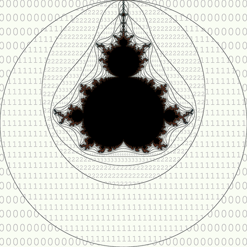
Figure 1. Escape time levels

We can also follow the same logic backwards. For every zₙ that ends up just barely outside the radius-2 circle there is an associated z_n-1 — the penultimate value of z before divergence. Taken together, these penultimate values form an roughly elliptic shape which gets transformed into a perfect circle by a single iteration of the Mandelbrot function. Assuming a large enough n we can continue this backtracking process to derive a series of outlines (known as lemniscates) that provide us with ever improving approximations of the true shape of the Mandelbrot set¹. When coloring based on the escape time these outlines are clearly visible as the boundaries of different shades of color. Instead of a traditional coloring, the accompanying image explicitly labels each region with its associated escape time.

The Boundary

Extrapolating this process into infinity would cause the fractally rough boundary to converge on the outline of the Mandelbrot set — which is the precise dividing line between divergent and non-divergent dynamics. Just like the fractal curves of a previous post this outline has a fractal dimension which exceeds its conventional one-dimensional nature. In 1991 a Japanese mathematician by the name of Mitsuhiro Shishikura proved that the Haussdorf dimension of the Mandelbrot boundary is exactly two which means that the outline is jagged enough to completely fill patches of two-dimensional space (just like the Hilbert curve). It is unfortunately beyond my mathematical capabilities to explain concisely why this is true so I will just leave a link to the paper in case you are interested.

The never-ending succession of outlines have also other remarkable properties. Despite their wiggliness the curves will always remain structurally equivalent with the initial circle: they will always remain contiguous and they will never get tied up in knots such that the curve would need to cross over itself, and furthermore two successive curves will never intersect each other. As a consequence the escape times of two adjacent depth bands are always at most one iteration apart — it is impossible to get from four to six without first going through five. Note that these assertions hold true as long as the initial circle has a radius of slightly more than two. Starting with a radius of exactly two would result in a discontinuity point at c=-2.

The implication of these properties is that whatever the precise shape of the infinitely detailed final curve may be it must necessarily enclose within itself a single fully connected area. In other words, there are no Mandelbrot "islands" – just one big continent with a nice two-dimensional coastline – which guarantees that it is always possible to travel from one interior location to another without ever having to get your feet wet. This property becomes even more striking when we start zooming deeper into the boundary and see that some of the routes are infinitely narrow. But first, let us set foot on the interior.

Main Cardioid

The most prominent feature of the interior is the "pierced circle" which is decorated by an infinite number of self-similar outgrowths later referred to as bulbs. Somewhat surprisingly the shape can be described exactly as what is known as a cardioid (a special case of an epicycloid). It is a shape which gets traced by a point fixed to the perimeter of a circle rolling around on the surface of another (stationary) circle of equal radius. In the case of Mandelbrot, both circles must have a radius of ¼, the stationary circle must be centered on c=0, and – to get the orientation right — the tracing point should start by touching the surface of the stationary circle at c=¼. The rest will follow.

Since both circles have the same radius the outer circle rolls around exactly once before returning to its initial position. Near the contact point this motion produces the sharp spike terminating at c=¼ (also known as the cusp) and its antipodal point at c=-¾. The nearest and farthest points from the inner circle respectively. The somewhat heart-shaped curve encloses within itself all values of c whose z sequences can be said to eventually converge on a single value. Although, since none of the values actually converge in finite time it would perhaps be more appropriate to talk about the rate of convergence. The rate is fastest near the center of the cardioid, but gradually slows down when approaching the cardioid boundary. These dynamics are primarily the result of the z² term of the Mandelbrot function.

Recall that complex multiplication (and thus squaring) can be represented as a combined rotation and scaling. Which in the polar coordinate form is the same as adding angles and multiplying distances. Complex values on the positive real axis have an argument (angle) of zero which means multiplying by such a number incurs no rotation. Likewise, whenever the absolute value (distance from zero) of a complex number is exactly one, multiplying by it incurs no scaling. By definition these transformational identities intersect at 1 which is to say that multiplying by one does not change the number being multiplied. The non-identity dynamics of distance squaring are also pretty straightforward: values less than one become smaller and values larger than one become bigger.

So the Mandelbrot question can be rephrased as: does the square term manage to reduce the absolute value as fast as we increase it when we add c? Up until to the pointy end of the cusp the answer is yes, and an equilibrium solution can be found where further iterations have no effect — which can be expressed mathematically as z²+c=z. However, past this point the delicate balance breaks and the dynamics undergo a phase shift from converging to diverging. For anything larger than c=¼ the value of z eventually becomes larger than one at which point the squaring no longer counterbalances the addition, but instead starts reinforcing it resulting in unbounded growth².

In the direction of the negative numbers this counterbalancing force is much more effective because of sign cancellation (which is effectively a 180° degree rotation). When we square the value -½ we not only halve its absolute value, but since we also flip the sign the effective value change (+¾) is three times larger in magnitude than in the case of +½ (-¼). It is thanks to this additional oomph that the boundary of the cardioid is further away from its center in the direction of the negative real numbers. Unfortunately, when we combine the dynamics of arbitrary rotation and scaling the end results become much harder to decipher. Although roughly speaking, the counterbalancing contribution of the rotational component comes from a kind of destructive interference whose effect is greatest along the negative real axis — where the set extends all the way to minus two.

Inner Color

In order to better explore the finer structure of the interior regions we need to ditch the ubiquitous escape time algorithm currently obscuring our view. Instead of visually ranking the relative instabilities of various c values it would be more appropriate to visualize their relative stability. As we already know, the dynamics of the interior are overwhelmingly periodical, especially if we also equate convergence with period-1 dynamics. For a z sequence to be perfectly periodical there should be no preperiodic lead-up phase which requires the sequence to keep returning to exactly zero at fixed intervals, where the length of the interval in number of iterations tells us the period of the sequence. However, since there are vastly more imperfectly periodical sequences than perfect ones it would be great if the coloring scheme allowed for some wiggle room.

One possibility would be to track the minimum absolute value of z. Perfectly periodical orbits would have a value of zero and it is not unreasonable to assume that values close to zero would correspond to near-perfect periodicity. Using this method some internal structure can indeed be revealed, but unfortunately this branch-like structure remains rather blurry and thus difficult to see. Luckily, it is possible to enhance the detail by instead tracking which n contributed the minimum absolute value³. This makes the value discrete instead of continuous and we effectively end up measuring the "approximate period" of the sequences. The methods can also be combined freely.

In the initial display mode areas with a small minimum absolute value are the brightest and areas where the resulting sequences never get close to zero are darker. The dark branches spreading out from the center present us with a new fractal pattern where each branch keeps recursively splitting into two as it approaches the edge of the cardioid. Each bulb around the cardioid seems to be situated at a point where two adjacent branch structures reconverge. The second 'period domain' display mode makes it obvious that these branching structures are actually the boundaries of different regions of "approximate period" making them in some sense analogous to the escape time level curves.

The (mostly) red pin marking the location of c is again freely movable, and whichever z (of n greater than zero) happens to have the smallest absolute value is colored green. In the period-1 domain this value will always be z₁, and since it is equal to c only one large pin (colored green) is shown. When c straddles a domain boundary there are two or more z values which have the same minimal absolute value and the "approximate period" of the orbit is in a kind of intermediate state. The last 'hybrid' display mode is designed to highlight the branching structure of these boundaries.

These branching structures visualize clearly that for c near the center of the cardioid the behaviour of resulting orbits is primarily dominated by the dynamics of absolute value squaring. Since squaring makes small absolute values even smaller the rate of convergence is high. However, as we move further away from the center the rotational dynamics start taking over with the lowest periodicities expressed first. When we reach the edge of the cardioid the scaling component is no longer able to "pull" the sequences to a single value and the dominance of the rotational component separates the different period orbits into bulbs of their own. We will investigate this structure in the next post in plentiful detail.

Main "disk"

Laying the groundwork for that investigation requires us to perform a certain mathematical trick. You don't necessarily need to know how the trick is performed, but if you are interested the appendix explains the setup. Be sure to click through its animations if nothing else! In short, by performing the trick (an illusion!) we can alter the shape of the Mandelbrot set so that it is a bit more agreeable to our analysis. Try clicking the button below and see how it changes the earlier demo.

The main cardioid of the Mandelbrot is now much friendlier and moreover perfectly round! The similarly transformed behaviour of the orbit lines reveals that something is not quite right as there is a rather abrupt transition as c crosses the positive real number line. In any case, the key thing to pay attention to is the correspondence between the different orbit periods and the argument value (or angle) of c. Just like before the period-2 dynamics manifest half a turn away from the positive real axis (at 180°) and the vicinity of positive real axis (near 0°) is mainly dominated by the period-1 dynamics — or in other words the dynamics of singular convergence.

More importantly though, all the other periods now align with angle values which are just as rationally distributed. The period-3 bulbs sprout at angles 120° and 240° away from the center equating to one third and two thirds of a turn. The period-5 bulbs are located at 72°, 144°, 216° and 288° corresponding to turn ratios of ⅕, ⅖, ⅗, and ⅘ respectively. You can probably pick up on the pattern. The only slight hitch is that one of the supposed values for period-4 would be ²⁄₄ which overlaps with period-2 behaviour. However, this need not discourage us since arguably period-4 dynamics are in some sense a manifestation of period-2 dynamics just with a different time scale (in terms of iterations). Since the ratio equivalences arise due to matters of divisibility, only prime numbered orbit periods are guaranteed not to overlap with "lower-order" dynamics.

Internal ray structures

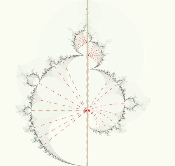
Drawing a set of angular rays within our new Mandelcircle and then undoing our earlier illusion allows us to visualize this phenomena within the original context of the cardioid. When the rays are curved in this manner they become known as the 'internal rays' of the main cardioid. Naturally, each smaller bulb around the main cardioid/circle has its own internal ray structures which point out the directions of the next smaller set of bulbs, and so on ad infinitum. We will investigate this recursive bulb structure in more detail in the next post.

Diving Deeper

So to summarize. Coloring based on sequence escape time is the ubiquitous way off visualizing the outside of the Mandelbrot set. The succession of escape time level curves that border the resulting color bands approach the Mandelbrot boundary as the number of iterations increases. Once we start zooming in we see how these patterns become more intricate the closer we get to the boundary never quite reaching it. Visualizing the interior is possible with other techniques which bring out other (perhaps less well-known) structures of the set and with some mathematical trickery these structures can be simplified to a surprising degree.

To be continued.

Appendix: Uncardioiding

As we have already learned, complex valued additions and multiplications are transformations in disguise so it should come as no surprise that other mathematical operations on the complex plane also behave like transformations. Recall the equilibrium equation which dominates the interior of the cardioid — z²+c=z. The equation can be rearranged to a slightly different form which essentially allows us to answer questions like: which value of c maintains an iterative equilibrium at this value of z? Posing the question in this way seems a bit backward in the context of the Mandelbrot, but we can turn things around if we invert the equation and solve for z instead.

How we arrive at the solution isn't all that important in our context, but the result can be easily verified by solving in the opposite direction. Just like addition and subtraction, or multiplication and division, these functions are the inverses of each other. The latter form allows us to now find the answers to a somewhat more relevant question: which value of z maintains an iterative equilibrium for a given value of c? It would be tempting to think that this is the same as finding the convergence point for any given c, but this holds true only within the cardioid. Outside the cardioid the sequences generated by c fail to "find" their perfect equilibrium point and instead diverge or settle on periodical cycles (as we already know). The reason for this perhaps unexpected change in behaviour is something worth investigating, but I will save it for another time.

The somewhat perplexing animations above attempt to visualize how these two functions transform the values they act upon, but instead of focusing on single values the functions are applied to entire patches of the complex plane at once. The initial animation starts by showing a square-shaped distribution of z values and as the animation progresses⁴ these values get turned into a differently shaped distribution of c values. During the animation the patch seems to fold in on itself so that the positive real line (downward blue) disappears almost entirely. In some sense it has actually turned into a parabola similar to the imaginary axis (red), but as the curving happens in a third dimension perpendicular to your screen it might be a bit hard to wrap your head around. The main feature of the transformation becomes more apparent if you change the coordinate mode by clicking on the left button — changing it from "Cartesian" to "Polar".

In the polar coordinate mode we see a half-radius circle (highlighted in blue) transform itself into a cardioid which just so happens to match the exact description of the Mandelbrot cardioid. The same folding of the complex plane is still happening, but with a different coordinate system the end result now looks something like an interference pattern. When following the animation in the reverse (or inverse) direction, we can deduce that the equilibrium z values corresponding to c values exactly on the cardioid boundary form a perfect circle with a radius of ½. This reveals the rather surprising feat achieved by the inverse function — the value it produces is the same value that is produced by an infinite number of Mandelbrot iterations! As long as we remain within the cardioid that is.

By clicking on the button on the right you can see the same animation with the inverse function ("c → z"). The transformation seems different, but this is only because we are setting the grid lines up differently. Previously they were laid out in "z-space", but now they are aligned with the inverse "c-space". What seems particularly concerning is that the inverse transformation seems to split part of the positive real axis in two leaving behind an unseemly gap! Appropriately though, the split coincides with the cusp coordinates of c=¼. The reason for the split was briefly alluded to in the footnotes of the complex number primer.

In the complex plane, when we square a number there are always two input values which give the same answer. The sign cancellation in the case of negative real numbers is the most obvious example, but the underlying effect works similarly across the whole domain of complex numbers — remember that negating a complex number is a essentially a 180° rotation. The folding behaviour of the forward function ("z → c") is the visual consequence of this duality. Every seemingly singular point in the output space is in fact composed of two input points which are brought together by the square-folding. Since a square root is defined to be the inverse of squaring it only makes sense then that each input value gives us two possible answers. Something which we conveniently glossed over in our previous definition. The third and final function of the animation ("c → ±z") visualizes what happens when we restore this symmetry.

Even after being made whole the inverse function exhibits a slightly unnerving dislocation, but once the twofold input space unfolds itself we can see that there are now two symmetric copies of the coordinate grid, each "glued" onto the real number line of its counterpart. This inverse function is precisely the mathematical trick we need in order to make the shape of the Mandelbrot set more agreeable. However, including both "branches" of the square root would make the shape a bit too agreeable so for the time being we settle for the asymmetric formulation displayed earlier. To get a sense of what the full unfolding looks like, go here and be sure to open the full image.

Time to go back and turn on the magic!